Superscalar Processor Design

Superscalar processors are designed to fetch and issue multiple instructions every machine cycle vs Scalar processors which fetch and issue single instruction every machine cycle.

ISA

• Instruction set architecture provides a contract between software and hardware i.e between program and the machine.
• ISA is an abstraction between the hardware implementation and programs can be written with knowledge of ISA.
• ISA ensures portability.
• For hardware developers, ISA is a specification.
• The set of instructions defined by ISA is an assembly language.
• Dynamic-static interface: defined as separation between stuff can be done statically (at compile time) and stuff can be done dynamically (at runtime).

Processor Performance is measured as CPI – cycles per instruction. There are following techniques for decreasing instruction count

• Executing multiple instructions per cycle using pipelining. The deeper pipeline goes, the branch misprediction penalty goes high as processor has to flush the pipeline and fill it up with new instructions. Also a deeper pipeline increases hardware and latency overhead.
• Decreasing the instruction count and moving the complexity on Hardware may increase cycle time.

Stages of Execution in Scalar Pipelined Processors

Image credit: http://www.oberle.org/procsimu-index.html

 

 

 

 

 

 

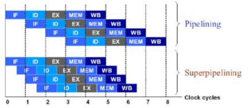
Stages in scalar Pipelined processors

1. Fetch: Since main memory is slow, the fetch stage is divided into two or more sub-stages. This ensures once the data/instructions starts coming into processor for execution, more than stage is executed in parallel. But since all the next stages are depend upon this stage, the pipeline is stalled until data/instructions become available at this stage. This stage is considered as in-order front-end.
   1. A superscalar processor can fetch more than one instruction in parallel.
2. Decode: The instructions are divided into further micro-instructions(micro-ops) at this level. Various caching and optimization techniques are done in order to complete this stage faster. This stage is considered as in-order front-end.
   1. for CISC processors this stage is complex and itself is divided into multiple substages.
   2. Since the decoding functionality is extremely complex, the predecoding has been implemented.
3. Dispatch:
4. Execution: the execution unit of a processor generally has more parallelism and considered as out of order execution stage. Intel x86 processors have 2 ALU, FPUs and vectorized processors in this stage.
5. Complete
6. Retite ( Writeback) : the results of processor execution are written back the registers.

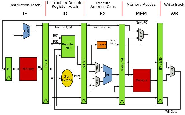
Image credit: By Inductiveload – Own work, Public Domain, https://commons.wikimedia.org/w/index.php?curid=5769084

The instruction types are

1. Arithmetic Operations
2. Load/store – data movement operations between memory, caches and registers.
3. Branch Instructions

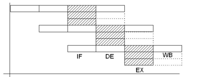
Superscalar Pipelines

This an example of a super scalar processor design. The pipeline is not only deep but also parallel.

Dynamic Pipelines

• Buffers are used to hold the data between multiple stages in the pipelined design.
• In parallel pipelined processors, multientry buffers are used.
• Parallel pipelined design that supports out of order execution of instructions is called as dynamic pipeline.
• The complex multientry buffer designs allow instructions flow in different order.
  • First of the buffers in pipeline is dispatch buffer. This buffer receives instructions from program in order but can dispatch them out of order to the functional units.
  • Similar kind of buffer named completion buffer is present at the back end of pipeline. It can receive results of computation in any order. This buffer retires the instructions in order and proceeds the results to WB stage.

Buffers in superscalar design

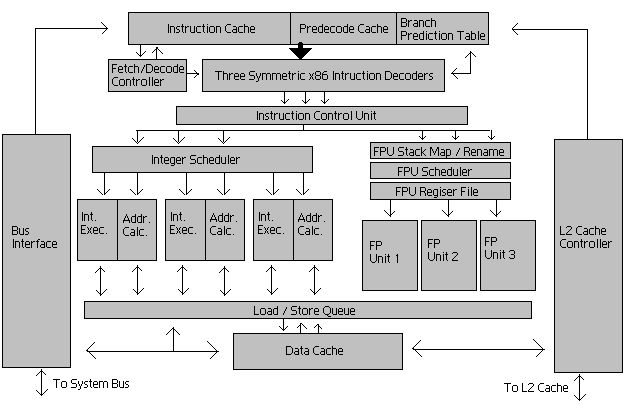
Example of latest Intel x86 Microprocessor

Each core has following number of hardware units:

• Reorder Buffer
  • ROB is used for register renaming and reordering the out of order execution results
  • 192 entries
• Reservation Station
  • has 60 entries
• Register file
  • 168 integer registers
• Vector registers
  • 168
• Loopback buffer
  • 56 entries.
• μop cache
  • 1536 μops, 8 way, 6 μop line size, per core
• L1I cache
  • 32 KB, 8 way set associative 64 sets
  • 64 bytes cache line
  • 32 bytes read and write per clock cycle
• L1D cache
  • 32 KB, 8 way set associative 64 sets
  • 64 bytes cache line
• L2 cache
  • 256KB, 8 way set associative 512 sets
  • 64 bytes cache line
• L3 cache
  • 45 MB (ring shaped shared)
• Instruction Fetch Rate
  • 16 bytes per clock cycle.

Trace Cache

After the instructions fetch, they are decoded and divided into μops. Instructions are stored in the trace cache after being decoded into μops. The opcode has length between 1 to 15.

Here is a nice video about breaking ISA instruction set.

Branch Prediction Techniques

Predicting branches correctly is important for superscalar processor performance. The branch prediction is much predictable because of various techniques explained below:

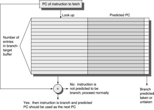
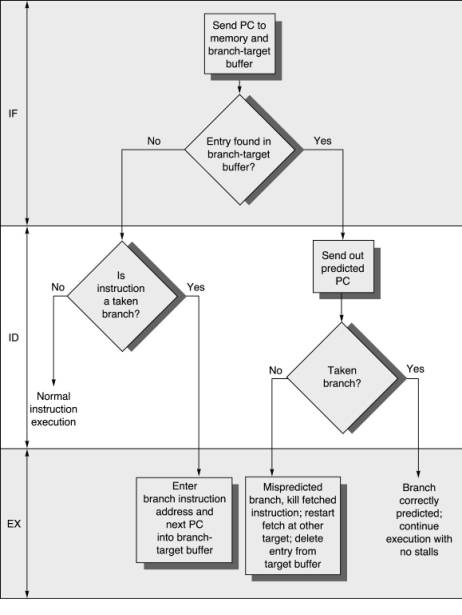
• Branch Target Speculation
  • A fully associative cache name Branch Target buffer is used for storing target address of last branch taken. For next lookup, the cache is used.
  • 
• Branch Conditional Speculation
  • Predictors based on hint from compiler
  • FSM: finite state machine based predictors

  • 

  • Real Life example PPC 604
    • BPU featuring dynamic branch prediction –
      • Speculative execution through two branches
      • 64-entry fully-associative branch target address cache (BTAC)
      • 512-entry branch history table (BHT) with two bits per entry for four levels of prediction— not-taken, strongly not-taken, taken, strongly taken.
• Multi-level adaptive branch predictor
• 
  • The Two-Level Branch Predictor, also referred to as Correlation-Based Branch Predictor, uses a two-dimensional table of counters, also called “Pattern History Table”. It was introduced by Yeh and Patt who because of the fact that the outcome of the branch depends not only on the branch address but also on the outcome of other recent branches (inter branch correlation) and a longer history of the same branch itself (intra branch correlation).
    • A Global Branch History is a shift register in which the outcome of any branch is stored. A “one” is stored for a taken branch and a “zero” for a non-taken one. The register is shifted through while storing the newest value. In order to address the table, the n last branch outcomes are considered.
    • The Local History Table is a table of shift registers of the sort of a global branch history. Each shift register, however, refers to the last outcomes of one single branch. Since this local history table is accessed as a one-level branch prediction table, it is not guaranteed that no overlapping of the branches occurs, and in one shift register may be stored the information of different branches.
    • Since the table has only two dimensions, two of the three information sources have to be selected to access rows and columns. Another method is to merge two sources to one, which will be covered later.
    • In general it can be stated that a two-level branch predictor is more accurate than a one-level branch predictor, but this advantage is also associated with the disadvantage of a more costly implementation and the fact that the so called Warm Up Phase, i.e. the time the table entries contain usable values, is much longer.

• Static Branch Prediction

  • Static Branch prediction algorithms do not speculate the prediction based on the past hence they are simple. Following are some of the techniques
    • Single Direction Prediction: speculate the direction is same for all the branches. Example: speculate branch is always taken or always not taken.
    • Backwards Taken/Forward not taken
    • Branch Hints: Compilers can hint the processor about possible branch output. Example:

    • __builtin_expect(argc,0)

    • Read more: https://stackoverflow.com/questions/14332848/intel-x86-0x2e-0x3e-prefix-branch-prediction-actually-used

• Dynamic Branch Prediction

  • Dynamic Branch prediction predicts at the rate of 80% to 95%.
  • The past outcomes are used as input for branch prediction.
    • One level branch predictor
    • Various predictor features
    • Two level branch predictor
    • Hashing techniques
    • Difficulties
    • Hybrid branch predictor
    • Multiple component Hybrid branch predictor
    • Branch classification
    • Industry branch prediction implementations

Register Renaming

Register renaming is controlled by the reorder buffer and the scheduler. Register renaming is a technique that eliminates the false data dependencies arising from the reuse of architectural registers by successive instructions that do not have any real data dependencies between them.

Machine language programs specify reads and writes to a limited set of registers specified by the instruction set architecture (ISA). For instance, the Alpha ISA specifies 32 integer registers, each 64 bits wide, and 32 floating-point registers, each 64 bits wide. These are the architectural registers